Getting started on PySpark on Databricks (examples included)

Gets python examples to start working on your data with Databricks notebooks.

Jean-Christophe BaeyOctober 02, 2019

Photo by Franz Harvin Aceituna on Unsplash

TL;DR;

This article will give you Python examples to manipulate your own data. The example will use the spark library called pySpark.

Prerequisites: a Databricks notebook

To get a full working Databricks environment on Microsoft Azure in a couple of minutes and to get the right vocabulary, you can follow this article:

Part 1: Azure Databricks Hands-on

Spark session

Databricks Notebooks have some Apache Spark variables already defined:

SparkContext: sc
- Spark Context is an object that tells Spark how and where to access a cluster.
SparkSession (Spark 2.x): spark
- Spark Session is the entry point for reading data and execute SQL queries over data and getting the results.
- Spark session is the entry point for SQLContext and HiveContext to use the DataFrame API (sqlContext).

All our examples here are designed for a Cluster with python 3.x as a default language. That's why we do not need the magic keyword %python on the first line. This is however required for Scala cells of our notebook.

print("Spark version", sc.version, spark.sparkContext.version, spark.version)
print("Python version", sc.pythonVer)

Same in Scala:

%scala
println("Spark version " + sc.version)
println("Spark version " + spark.version)
println("Spark version " + spark.sparkContext.version)
println("Scala version " + scala.util.Properties.versionString)

RDD (schema-less) vs DF

RDD: Resilient Distributed Dataset (RDD)

An RDD is an immutable distributed collection of data partitioned across nodes in your cluster with a low-level API. It is schema-less and used for low-level transformation and actions.

Dataframe (DF)

A DataFrame is a distributed collection of rows under named columns. It is the same as a table in a relational database. It is closed to Pandas DataFrames. A DataFrame has the ability to handle petabytes of data and is built on top of RDDs. A DataFrame is mapped to a relational schema.

Create a RDD

myRDD = sc.parallelize(
    [('Amber', 22), ('Alfred', 23), ('Skye',4), ('Albert', 12), 
     ('Amber', 9)])

Display the content of the RDD

# Option 1
print(myRDD.collect())

# Option 2
for row in myRDD.take(myRDD.count()): print(row)

Convert a RDD to a DF

You need to give the schema to use:

from pyspark.sql import types

DFSchema = types.StructType([
  types.StructField('name', types.StringType()),
  types.StructField('age', types.LongType())
])

# 3 ways to convert the RDD to a DF:
df1 = spark.createDataFrame(myRDD, DFSchema)
df2 = myRDD.toDF(DFSchema)
df3 = myRDD.toDF(['name','age'])

Display the dataframe content (first 1000 rows)

display(df1)

Display the DF schema

df1.printSchema()

The number of rows

df1.count()

The column names

df1.columns

The number of partitions

The dataframe is divided in partitions. Each time an evaluation is requested, a job is created and the DF is distributed among workers on the cluster. The entity that is distributed to each worker is a partition. The number of partitions is defined automatically and can also be set by hand. It is recommended to adjust the number of partitions especially to reduce it if you do have a very small dataframe. In that case, the data distribution will add an overhead.

# Get the partition number
print("Partitions", df1.rdd.getNumPartitions())

# Set the number of partition (re-repartition)
df1 = df1.repartition(2)

Alias the DF in the SQL context

df1.createOrReplaceTempView("user")

Perform SQL queries

Embedded in Python

result_df = spark.sql("SELECT * from user")

In a SQL cell

%sql

SELECT * from user

Examples of DF queries

display(df1.select("name", "age").where("name = 'Amber'"))

display(df1.select("name", "age").where("name = 'Amber'"))

from pyspark.sql import functions as F

display(df1.select("*").where(F.col("name").eqNullSafe("Amber")))

display(df1.select("name", "age").where(F.col("name").eqNullSafe("Amber")))

display(df1.select(*df1.columns).where(F.col("name").eqNullSafe("Amber")))

display(df1.select(F.min("age").alias("minValue"), F.max("age")))

Regular python interactions

Get the DF in regular python list

pythonRegularObject = df1.collect()

Destructuring the result in regular Python variables

minValue, maxValue, = df1.select(F.min("age"), F.max("age")).head()

print("Min: {}, Max: {}".format(minValue, maxValue))

Same in Scala

%scala

import org.apache.spark.sql.functions._

var df = spark.table("user")
// df = spark.sql("select * from user")

var Row(minValue, maxValue) = df.select(min("age"), max("age")).head
  
println(s"Min: ${minValue}, Max: ${maxValue}")

User Defined Functions (UDF)

Without UDF

result_df = df1.select("name", "age", (F.col("age") * 2).alias("ageX2"))

display(result_df)

With an UDF

@udf("long")
def multiplyBy2(age):
  return age * 2

result_df = df1.select("name", "age", multiplyBy2("age").alias("ageX2"))

display(result_df)

Important note: avoid UDF as much as you can as they are slow (especially in Python) compared to native pySpark functions.

DF to RDD and vise versa (map, flatmap)

Applying a python function on each row thanks to the RDD function map to create a new column ageX2:

from pyspark.sql import Row

def tranformRow(row):
  newAge = row.age * 2
  return Row(name=row.name, age=row.age, ageX2=newAge)
  # return Row(**{"name": row.name, "age": row.age, "ageX2": newAge})

result_df = df1.rdd.map(tranformRow).toDF()

display(result_df)

Advanced example using Python generator (yield keyword) and flatmap to create new rows:

# Advanced

def rowExpander(x):
  yield Row(**{"name": x.name, "age": x.age})
  yield Row(**{"name": x.name, "age": x.age * 2})
  
result_df = df1.rdd.flatMap(rowExpander).toDF()

display(result_df)

RDD api can also be used to get back regular python array:

df1.select("name").distinct().rdd.flatMap(lambda x: x).collect()

File handling

Magic `%fs`

Use the %fs magic keyword:

%fs

ls /mnt

Loading a JSON file

Load a Json file (the schema will be inferred)

# Option 1
df = spark.read.format("json").load("dbfs:/mnt/my_file.json")

# Option 2
df = spark.read.json("dbfs:/mnt/my_file.json")

You can speed up the JSON loading by providing the schema:

from pyspark.sql.types import *

dfSchema = StructType([
  StructField("id",LongType(),True),
  StructField("timestamp",LongType(),True),
  StructField("message",StringType(),True),
  StructField("signals",ArrayType(StructType(
      [
      StructField("key",StringType(),True),
      StructField("value",DoubleType(),True)
      ]),True),True)
])

# Providing schema speed up the loading
df = spark.read.format("json").schema(dfSchema).load("dbfs:/mnt/my_file.json")
display(df.limit(5))

A lot of different file formats are supported (CSV, JSON, Parquet, ORC, etc...).

DF handling examples

Explode

If you have a JSON file where each JSON is a row like this:

{
  "id": 1,
  "timestamp": 0001,
  "message": "message1",
  "signals": {
    "prop1": "value1",
    "prop2": "value2",
  }
}

{
  "id": 2,
  "timestamp": 0002,
  "message": "message2",
  "signals": {
    "prop3": "value3",
    "prop4": "value4",
  }
}

You can use the explode function to convert it into a DF like this:

id | timestamp | message  | key   | value
1  | 0001      | message1 | prop1 | value1 
1  | 0001      | message1 | prop2 | value2 
2  | 0002      | message2 | prop3 | value3 
2  | 0002      | message2 | prop4 | value4

dfExploded = (
  df.select("id", "timestamp", "message", F.explode("signals").alias("signal"))
  .select("id", "timestamp", "message", F.col("signal.key").alias("key"), F.col("signal.value").alias("value"))
)


display(dfExploded.limit(5))

display(dfExploded.filter("message='message1'"))

group by

ret = (
  dfExploded
  .filter("message='message1'")
  .groupBy("key")
  .agg(F.mean("value"))
)

display(ret)

Cache result to speed up further processing

intermediateDF = dfExploded.filter("message='message1'").cache()

Pivot


ret = (
  intermediateDF
  .groupBy("timestamp")
  .pivot("key", ["prop1", "prop2"])
  .agg(F.first("value"))
)

display(ret)

Plotting

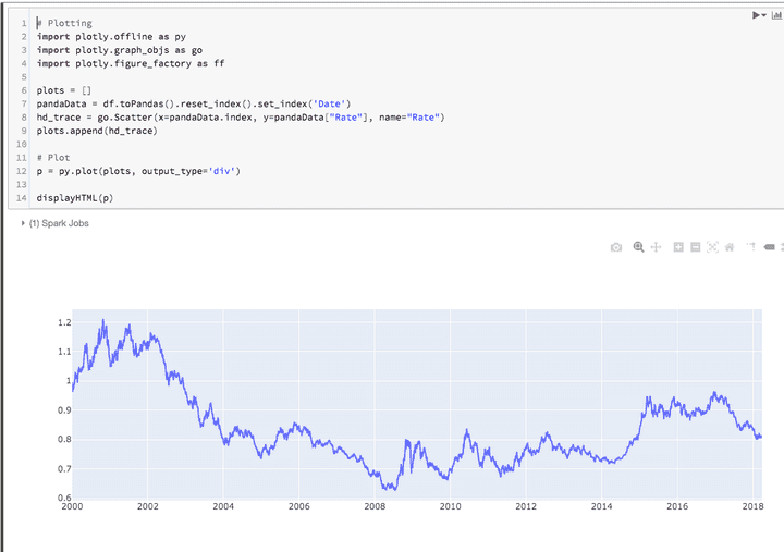
There is some built-in plotting with Databricks. However if you want more control, you can use external library like plotly](https://plot.ly/).

Getting some data to plot:

import requests
r = requests.get("https://timeseries.surge.sh/usd_to_eur.csv")
df = spark.read.csv(sc.parallelize(r.text.splitlines()), header=True, inferSchema=True)
display(df)

Using plotly

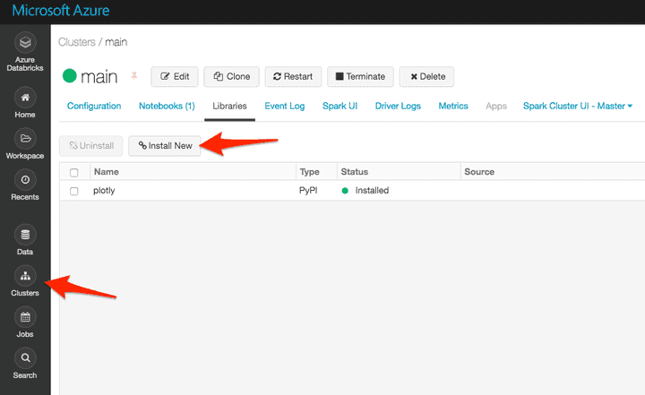
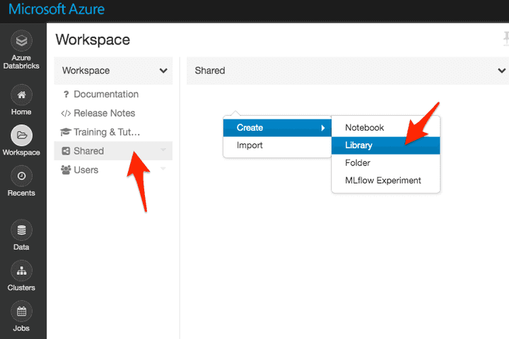
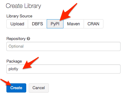
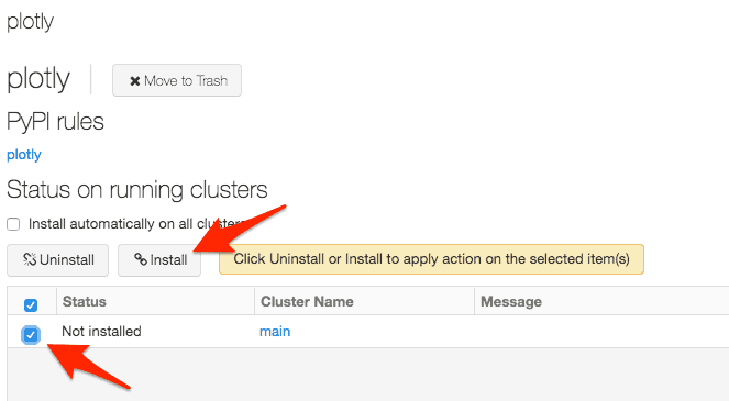
Important note: you need to add plotly as a cluster dependency:

Option 1

Option 2

# Plotting
import plotly.offline as py
import plotly.graph_objs as go
import plotly.figure_factory as ff

plots = []
pandaData = df.toPandas().reset_index().set_index('Date')
hd_trace = go.Scatter(x=pandaData.index, y=pandaData["Rate"], name="Rate")
plots.append(hd_trace)
 
# Plot  
p = py.plot(plots, output_type='div')

displayHTML(p)

Windows

We will create a tumbling window to downsample the data to 1 point every 30 days.
We will use the mean function.

tumblingSize = "30 days"

downsampledDf = (
  df
  .groupBy(F.window("Date", tumblingSize).alias("timestamp"))
  .agg(F.mean("Rate").alias("Rate"))
   .select(F.col("timestamp.start").alias("Date"), "Rate")
   .sort(F.asc("Date"))
)

display(downsampledDf)

Plot again:

plots = []
pandaData = downsampledDf.toPandas().reset_index().set_index('Date')
hd_trace = go.Scatter(x=pandaData.index, y=pandaData["Rate"], name="Rate")
plots.append(hd_trace)
 
# Plot  
p = py.plot(plots, output_type='div')

displayHTML(p)

👉 Don't forget to follow me on Twitter to be notified when new posts are available!

Follow @jcbaey